
Autoencoders
Implementation of a denoised Autoencoder

An AutoEncoder (AE) is a neural network design comprising two interconnected networks: Encoder and Decoder. The Encoder takes in the input an image and transforms it into a lower-dimensional latent spatial vector. Subsequently, the Decoder reconstructs this vector to generate an output closely resembling the initial input. Throughout this process, the network is trained. The purpose of Autoencoders is to learn low-dimensional feature representations of the input data.

Denoising autoencoders exhibit versatility across various domains or application areas, often requiring slight adjustments based on the nature of the dataset being utilized. In this tutorial, we will explore one such variant known as convolutional denoising autoencoders, specifically designed for denoising image data.
These models take a noisy image as input and employ multiple convolutional operations to extract crucial features. These latent features are then fed into a series of deconvolutional layers to reconstruct a cleaner version of the image, maintaining the same height and width.
Implementation of an Autoencoder
The implementation of a basic AE consisted on a network architecture densely connected layers as follow:
Layer 1: 128 Neurons with ReLU activations
Layer 2: 64 Neurons with ReLU activations
Layer 3: 32 Neurons with ReLU activations
Layer 4: 64 Neurons with ReLU activations
Layer 5: 128 Neurons with ReLU activations
Layer 6: 784 Neurons with Sigmoid activation
On this AE, I’ve use the Rectified Linear Unit (ReLU) activation functions for the input and hidden layers and a Sigmoid function as the output layer of the Artificial Neural Network (ANN).
The ReLU function returns 0 if it receives any negative input, but for any positive value x, it returns the value back. In practice it is fast to compute, hence it has become the most used activation function on ANNs.
The sigmoid function is a special form of the logistic function. This function is used as an output layer when you want to guarantee that the predictions will always fall within a given range of values, 0 to 1.
Weights Initializer
During the process of constructing the AE, the TensorFlow initializer RandomNormal was used on the initial experiments. But it was noticed that after the first epoch, the output matrix of the sigmoid layer was containing NaN values. This occurs due a saturation of the sigmoid function. A typical solution for this is problem is use another initialiser that solves this problem or implement a sigmoid function that is numerical stable. On my case I resulting using the HeNormal initialiser provided by TensorFlow.
Optimizer
The Adaptive moment estimation (Adam), is an adaptive learning rate algorithm for first-order gradient-based optimisation. It is computationally efficient and has a little memory footprint.
This was the optimizer utilized to update the weights for the AE during training phase. It requires less tuning of the learning rate hyperparameter. The default learning rate η=0.001 has been used.
Here is an illustrative diagram presenting the key components involved on the training phase of an Artificial Neural Network.

Results
The code that implement this AutoEncoder using the popular MNIST dataset can be found here. On this case we wanted to show how to implement a Class using Keras.
The main goal of the training gradient-based phase is to reduce the loss. The loss values across 200 epochs is shown in the following image.

It is noticed how the model was making improvements on each iteration. It was noticed that after around epoch 70-80 the model was not making any more significant improvement. The final loss obtained after 200 epochs was 0.0479.
In order to evaluate the performance of the model in a visual manner. A group of 3 randoms data points (images) were selected from the test dataset and a visualisation of the original, noisy and reconstructed image were generated.

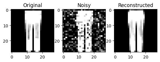

It's evident that the model demonstrates good performance, effectively reconstructing a nearly identical image from a noisy input.